Welcome to my Math Imaging Code Library!
If you are reading this, you probably got here from GitHub. These pages contain the documentation of some of the mathematical image processing routines I’ve written during my PhD. All codes require either NumPy, SciPy or matplotlib to be installed on your system.
I have coded these modules a while ago and most of them have not been updated since - so please use with caution. That said if you find bugs or have suggestions/comments please do not hesitate to contact .
Note: These pages contain documentation only, to download the source code, please refer to my corresponding GitHub repository.
The following table provides a brief overview of available routines sorted by application area.
| Applications | Routines | Brief Description |
| Mathematical Image Processing | Chambolle’s Algorithm | Chambolle’s Algorithm for TV denoising |
| Ambrosio–Tortorelli Algorithm | Ambrosio–Tortorelli algorithm to solve the Mumford-Shah segmentation problem | |
| Image Manipulation | Load/Save/Show Image | Image manipulation in Python |
| Construct Images | Create prototype test images | |
| Miscellaneous | Numerical Differentiation | Assemble discrete differential operators |
| Visualization of Vector Fields | Plot 2D vector fields |
Image Processing Algorithms
The following routines are Python implementations of a denoising and a segmentation algorithm.
Chambolle’s Algorithm
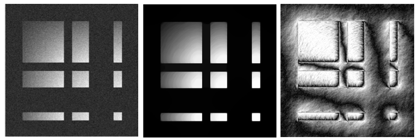
Exemplary approximate solution to the total variation denoising problem computed by Chambolle’s projection algorithm. An artificial test image (compare Construct Images) was corrupted by 5% additive Gaussian noise (left). The middle panel shows the denoised image obtained by using Chambolle’s approach, the \(L^1\)-norm of the associated dual variable is shown in the right panel.
An implementation of Chambolle’s projection algorithm to numerically approximate a solution of the Rudin–Osher–Fatemi total variation denoising problem.
chambolle(ut[, Dx, Dy, mu, dt, itmax, tol]) |
Solve the nonlinear TV-denoising problem using Chambolle’s projection algorithm |
Ambrosio–Tortorelli Segmentation Algorithm
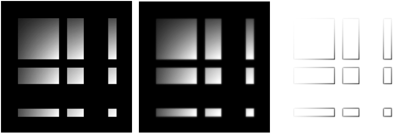
Exemplary Ambrosio–Tortorelli segmentation of the bars image (compare Construct Images).
Shown are the original image (left), the computed approximation (middle) and the
associated phase function (right).
An algorithmic approach to numerically approximate a minimizer of the Ambrosio–Tortorelli functional which itself approximates the Mumford–Shah cost functional for image segmentation.
myat(f, ep[, nu, de, la, tol, itmax, iplot, ...]) |
Solve the Ambrosio–Tortorelli approximation of the Mumford–Shah functional |
Image Manipulation Tools
The modules below provide various routines for the creation, manipulation and export of images (represented as NumPy arrays) in Python.
Load/Save/Show Images
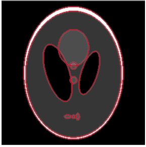
An edge map of the phantom image (compare Construct Images) visualized as red overlay
using the function blendedges()
Routines to read, write and show images (stored as NumPy arrays).
imwrite(figobj, fstr[, dpi]) |
Save a Matplotlib figure camera-ready using a “tight” bounding box |
normalize(I[, a, b]) |
Re-scale a NumPy ndarray |
blendedges(Im, chim) |
Superimpose a (binary) edge set on an gray-scale image using Matplotlib’s imshow |
recmovie([figobj, movie, savedir, fps]) |
Save Matplotlib figures and generate a movie sequences |
Create Prototype Test Images
A collection of handy routines to load or construct test images with specific properties.
onesquare(N[, ns]) |
Create a simple piece-wise constant gray-scale image: a white square on a black background |
fivesquares(N[, ns]) |
Create a piece-wise constant gray-scale image: five squares of different intensities on black background |
spikes(N[, ns]) |
Create a piece-wise linear gray-scale image of four squares with gradually increasing intensities |
bars(N[, ns]) |
Create a piece-wise linear gray-scale image of rectangles with gradually increasing intensities |
manysquares(N[, ns]) |
Create a piece-wise linear gray-scale image of 16 squares with gradually increasing intensities |
tgvtest(N[, ns]) |
Create a gray-scale image consisting of one shaded square often used to illustrate TV denoising problems |
myphantom(N[, ns]) |
Create the famous Shepp–Logan phantom |
gengrid(N) |
Creates an N-by-N grid needed to construct most artificial images |
Miscellaneous
Two modules that might come in handy when constructing approximations of 2D differential operators on regular grids or when working with 2D vector fields.
Numerical Differentiation using Finite Differences
Routines to numerically approximate first order differential operators on regular grids using finite differences.
fidop2d(N[, drt, fds]) |
Compute 2D finite difference operators |
myff2n(n) |
Give factor settings for a two-level full factorial design |
Visualization of Two-Dimensional Vector Fields
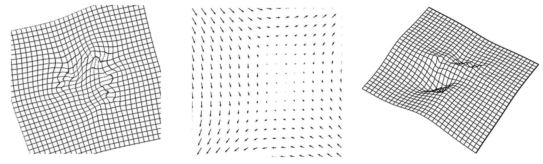
Three different visualizations of a two-dimensional vector field obtained by using the routines
mygrid() (left), myquiv() (middle) and mywire() (right).
Easy-to-use wrappers for Matplotlib functions generally employed to plot 2D vector fields defined on regular grids.
myquiv(u, v) |
Plots a 2D vector field using “sane” defaults for Matplotlib’s quiver. |
makegrid(N[, M, xmin, xmax, ymin, ymax]) |
Create an M-by-N grid on the 2D-domain [xmin,xmax]-by-[ymin,ymax] |
mygrid(u, v[, x, y, rowstep, colstep, ...]) |
Plot a 2D vector field as deformed grid on a 2D lattice |
mywire(u, v[, x, y, rowstep, colstep]) |
Plot a 2D vector field as 3D wire-frame using Matplotlib’s plot_wireframe |